Archetypal Analysis

Introduction

In this vignette, we present

1. a brief overview of the theory behind archetypal analysis

2. a description of the optimization procedure used in our implementation

3. a guide to using the AA class and its AA.fit() method

Mathematical Setup (Notation and Objective)

We use the same notation as in the supplementary methods:

• \(N\): number of samples (cells), \(D\): embedding dimensions, \(K\): number of archetypes

• \(\mathbf{X} \in \mathbb{R}^{N \times D}\): data matrix (row \(n\) is \(\mathbf{x}_n^T\))

• \(\mathbf{A} \in \mathbb{R}^{N \times K}\): sample-to-archetype coefficients

• \(\mathbf{B} \in \mathbb{R}^{K \times N}\): archetype-to-sample coefficients

• \(\mathbf{Z} \in \mathbb{R}^{K \times D}\): archetype matrix

Archetypal analysis assumes

\[ \hat{\mathbf{X}} = \mathbf{A}\mathbf{Z}, \qquad \mathbf{Z} = \mathbf{B}\mathbf{X}. \]

With row-stochastic constraints,

\[ F(n,m) := \{\mathbf{H} \in \mathbb{R}^{n \times m} \mid \mathbf{H} \ge 0,\; \mathbf{H}\mathbf{1}_m = \mathbf{1}_n\}, \]

the optimization problem is

\[ \hat{\mathbf{A}}, \hat{\mathbf{B}} = \arg\min_{\mathbf{A} \in F(N,K),\; \mathbf{B} \in F(K,N)} \left\|\mathbf{X} - \mathbf{A}\mathbf{B}\mathbf{X}\right\|_F^2. \]

Important properties used below: the objective is translation/scale invariant in \(\mathbf{X}\) and biconvex in \((\mathbf{A},\mathbf{B})\).

First, we will import some package that we need throughout this vignette.

from datetime import datetime
import partipy as pt
import numpy as np
import matplotlib.pyplot as plt

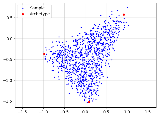
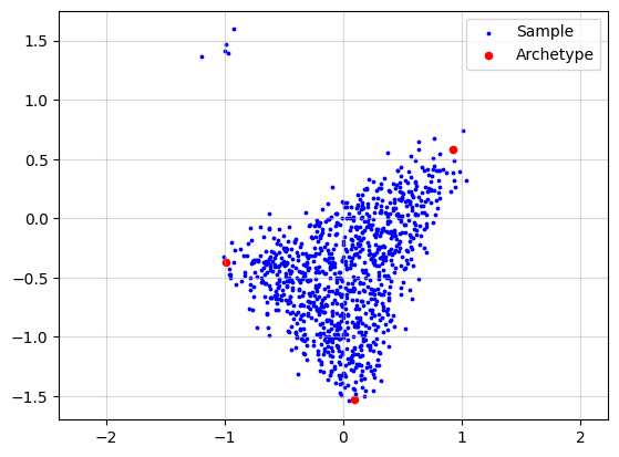
Now, we simulate a dataset to provide an intuitive explanation of archetypal analysis. To make the simulation more realistic, we add noise to each data point by sampling a noise vector from an isotropic Gaussian distribution.

X, A, Z = pt.simulate_archetypes(n_samples=1_000, n_archetypes=3, n_dimensions=2,
                                 noise_std=0.10, seed=123)
print(f"{X.shape}")
print(f"{A.shape}")
print(f"{Z.shape}")

(1000, 2)
(1000, 3)
(3, 2)

plt.grid(alpha=0.5)
plt.scatter(x=X[:, 0], y=X[:, 1], s=3, c="blue", label="Sample")
plt.scatter(x=Z[:, 0], y=Z[:, 1], s=20, c="red", label="Archetype")
plt.legend()
plt.axis("equal")
plt.show()

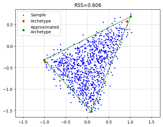
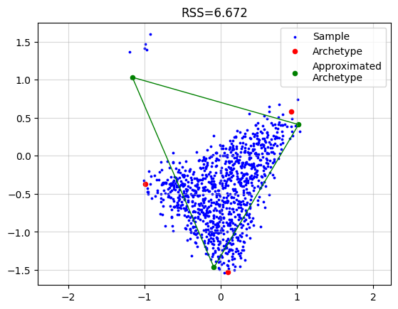
Standard Archetypal Analysis

For standard archetypal analysis, we solve

\[ \hat{\mathbf{A}}, \hat{\mathbf{B}} = \arg\min_{\mathbf{A} \in F(N,K),\; \mathbf{B} \in F(K,N)} \left\|\mathbf{X} - \mathbf{A}\mathbf{B}\mathbf{X}\right\|_F^2 \]

with alternating updates:

\[ \mathbf{A} \leftarrow \arg\min_{\mathbf{A} \in F(N,K)} \|\mathbf{X}-\mathbf{A}\mathbf{Z}\|_F^2, \qquad \mathbf{B} \leftarrow \arg\min_{\mathbf{B} \in F(K,N)} \|\mathbf{X}-\mathbf{A}\mathbf{B}\mathbf{X}\|_F^2, \qquad \mathbf{Z}=\mathbf{B}\mathbf{X}. \]

In this notebook, pt.AA(...) executes this procedure (with solver-specific updates under simplex constraints).

AA_object = pt.AA(n_archetypes=3)
AA_object.fit(X)
Z_hat = AA_object.Z

plt.grid(alpha=0.5)
plt.scatter(x=X[:, 0], y=X[:, 1], s=3, c="blue", label="Sample")
plt.scatter(x=Z[:, 0], y=Z[:, 1], s=20, c="red", label="Archetype")
plt.scatter(x=Z_hat[:, 0], y=Z_hat[:, 1], s=20, c="green", label="Approximated\nArchetype")
Z_loop = np.vstack([Z_hat, Z_hat[0]])
plt.plot(Z_loop[:, 0], Z_loop[:, 1], c="green", linestyle='-', linewidth=1)
plt.title(f"RSS={AA_object.RSS:.3f}")
plt.legend()
plt.axis("equal")
plt.show()

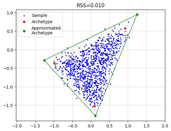
Relaxation of Convex Constraint on Archetypes

With delta > 0, ParTIpy relaxes the strict convex-hull constraint on archetypes. A convenient formulation is

\[ \min_{\mathbf{A} \in F(N,K),\; \mathbf{B} \in F(K,N),\; \boldsymbol{\alpha} \in [1-\delta,1+\delta]^K} \left\|\mathbf{X} - \mathbf{A}\,\operatorname{diag}(\boldsymbol{\alpha})\,\mathbf{B}\mathbf{X}\right\|_F^2, \]

with archetypes

\[ \mathbf{Z} = \operatorname{diag}(\boldsymbol{\alpha})\,\mathbf{B}\mathbf{X}. \]

Setting \(\delta=0\) recovers standard archetypal analysis. This relaxation follows the formulation introduced in [MH12] and has been used in downstream ParTI applications [KSH+15].

AA_object = pt.AA(n_archetypes=3, delta=0.25)
AA_object.fit(X)
Z_hat = AA_object.Z

plt.grid(alpha=0.5)
plt.scatter(x=X[:, 0], y=X[:, 1], s=3, c="blue", label="Sample")
plt.scatter(x=Z[:, 0], y=Z[:, 1], s=20, c="red", label="Archetype")
plt.scatter(x=Z_hat[:, 0], y=Z_hat[:, 1], s=20, c="green", label="Approximated\nArchetype")
Z_loop = np.vstack([Z_hat, Z_hat[0]])
plt.plot(Z_loop[:, 0], Z_loop[:, 1], c="green", linestyle='-', linewidth=1)
plt.title(f"RSS={AA_object.RSS:.3f}")
plt.legend()
plt.axis("equal")
plt.show()

Robust Archetypal Analysis

ParTIpy’s robust mode uses an iterative reweighting scheme (IRLS-like), following robust archetypal analysis ideas from [EL11]. In iteration \(t\), with sample weights \(\mathbf{w}^{(t)}\) and \(\mathbf{W}^{(t)}=\operatorname{diag}(\mathbf{w}^{(t)})\), the implemented updates are:

\[ \mathbf{A}^{(t+1)} \leftarrow \arg\min_{\mathbf{A}\in F(N,K)} \left\|\mathbf{W}^{(t)}\mathbf{X} - \mathbf{A}\mathbf{Z}^{(t)}\right\|_F^2, \]

\[ \mathbf{B}^{(t+1)} \leftarrow \arg\min_{\mathbf{B}\in F(K,N)} \left\|\mathbf{X} - \mathbf{A}^{(t+1)}\mathbf{B}\,\mathbf{W}^{(t)}\mathbf{X}\right\|_F^2, \qquad \mathbf{Z}^{(t+1)} = \mathbf{B}^{(t+1)}\mathbf{W}^{(t)}\mathbf{X}. \]

Then residuals are recomputed on the original scale,

\[ \mathbf{A}_0^{(t+1)}\leftarrow\arg\min_{\mathbf{A}\in F(N,K)}\left\|\mathbf{X}-\mathbf{A}\mathbf{Z}^{(t+1)}\right\|_F^2, \qquad \mathbf{R}^{(t+1)} = \mathbf{X}-\mathbf{A}_0^{(t+1)}\mathbf{Z}^{(t+1)}, \]

and weights are updated as \(\mathbf{w}^{(t+1)} = \omega(\mathbf{R}^{(t+1)})\) (e.g. bisquare, huber).

In the bisquare option below, strong outliers are down-weighted toward zero.

To demonstrate this behavior, we now add synthetic outliers.

n_outliers = 5
outlier_mean = np.array([-1.0, 1.5])
X_wo = np.zeros((X.shape[0]+n_outliers, X.shape[1]))
X_wo[:X.shape[0], :] = X.copy()
rng = np.random.default_rng(seed=42)
X_wo[X.shape[0]:, :] = rng.normal(loc=outlier_mean, scale=(0.1, 0.1), size=(n_outliers, 2))

print(f"{X_wo.shape}")
print(f"{A.shape}")
print(f"{Z.shape}")

(1005, 2)
(1000, 3)
(3, 2)

plt.grid(alpha=0.5)
plt.scatter(x=X_wo[:, 0], y=X_wo[:, 1], s=3, c="blue", label="Sample")
plt.scatter(x=Z[:, 0], y=Z[:, 1], s=20, c="red", label="Archetype")
plt.legend()
plt.axis("equal")
plt.show()

Now if we just run the standard algorithm we obtain.

AA_object = pt.AA(n_archetypes=3)
AA_object.fit(X_wo)
Z_hat = AA_object.Z

plt.grid(alpha=0.5)
plt.scatter(x=X_wo[:, 0], y=X_wo[:, 1], s=3, c="blue", label="Sample")
plt.scatter(x=Z[:, 0], y=Z[:, 1], s=20, c="red", label="Archetype")
plt.scatter(x=Z_hat[:, 0], y=Z_hat[:, 1], s=20, c="green", label="Approximated\nArchetype")
Z_loop = np.vstack([Z_hat, Z_hat[0]])
plt.plot(Z_loop[:, 0], Z_loop[:, 1], c="green", linestyle='-', linewidth=1)
plt.title(f"RSS={AA_object.RSS:.3f}")
plt.legend()
plt.axis("equal")
plt.show()

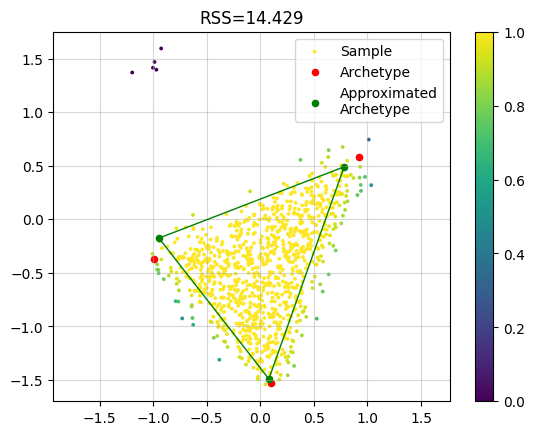
However, if we use the robust implementation we get a much better result. In the plot we colored each sample by the final weight. We see that the outlier samples have zero weight.

AA_object = pt.AA(n_archetypes=3, weight="bisquare", early_stopping=False)
AA_object.fit(X_wo)
Z_hat = AA_object.Z

plt.grid(alpha=0.5)
plt.scatter(x=X_wo[:, 0], y=X_wo[:, 1], s=3, c=AA_object.W, label="Sample")
plt.scatter(x=Z[:, 0], y=Z[:, 1], s=20, c="red", label="Archetype")
plt.scatter(x=Z_hat[:, 0], y=Z_hat[:, 1], s=20, c="green", label="Approximated\nArchetype")
Z_loop = np.vstack([Z_hat, Z_hat[0]])
plt.plot(Z_loop[:, 0], Z_loop[:, 1], c="green", linestyle='-', linewidth=1)
plt.title(f"RSS={AA_object.RSS:.3f}")
plt.legend()
plt.colorbar()
plt.axis("equal")
plt.show()

Coresets

For large \(N\), we can optimize on a weighted subset (coreset) \(\tilde{\mathbf{X}} \in \mathbb{R}^{\tilde{N} \times D}\) with \(\tilde{N} \ll N\):

\[ \hat{\mathbf{A}}, \hat{\mathbf{B}} = \arg\min_{\mathbf{A} \in F(\tilde{N},K),\; \mathbf{B} \in F(K,\tilde{N})} \left\|\mathbf{W}\tilde{\mathbf{X}} - \mathbf{W}\mathbf{A}\mathbf{B}\tilde{\mathbf{X}}\right\|_F^2, \]

where \(\mathbf{W}\) is diagonal. In the current implementation, its diagonal entries are the square roots of coreset weights.

After convergence on the coreset, \(\mathbf{A}\) is recomputed on the full dataset with fixed \(\mathbf{Z}=\mathbf{B}\tilde{\mathbf{X}}\). This follows the AA coreset construction in [MB19], which adapts lightweight coreset ideas from [BLK18].

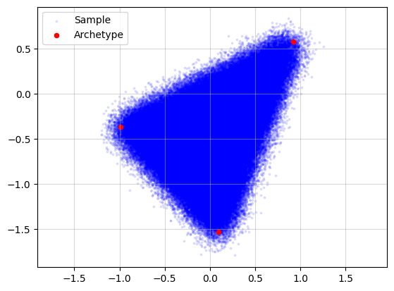
Let’s use the same underlying archetypes but generate many more samples to illustrate the computational effect.

X, A, Z = pt.simulate_archetypes(n_samples=200_000, n_archetypes=3, n_dimensions=2, 
                                 noise_std=0.10, seed=123)
print(f"{X.shape}")
print(f"{A.shape}")
print(f"{Z.shape}")

(200000, 2)
(200000, 3)
(3, 2)

plt.grid(alpha=0.5)
plt.scatter(x=X[:, 0], y=X[:, 1], s=3, c="blue", label="Sample", alpha=0.1)
plt.scatter(x=Z[:, 0], y=Z[:, 1], s=20, c="red", label="Archetype")
plt.legend()
plt.axis("equal")
plt.show()

Running archetypal analysis now takes quite some time

start = datetime.now()
AA_object = pt.AA(n_archetypes=3)
AA_object.fit(X)
Z_hat = AA_object.Z
end = datetime.now()
time = (end - start).total_seconds()

plt.grid(alpha=0.5)
plt.scatter(x=X[:, 0], y=X[:, 1], s=3, c="blue", label="Sample")
plt.scatter(x=Z[:, 0], y=Z[:, 1], s=20, c="red", label="Archetype")
plt.scatter(x=Z_hat[:, 0], y=Z_hat[:, 1], s=20, c="green", label="Approximated\nArchetype")
Z_loop = np.vstack([Z_hat, Z_hat[0]])
plt.plot(Z_loop[:, 0], Z_loop[:, 1], c="green", linestyle='-', linewidth=1)
plt.title(f"Time (s)={time:.2f} | RSS = {AA_object.RSS:.3f}")
plt.legend()
plt.axis("equal")
plt.show()

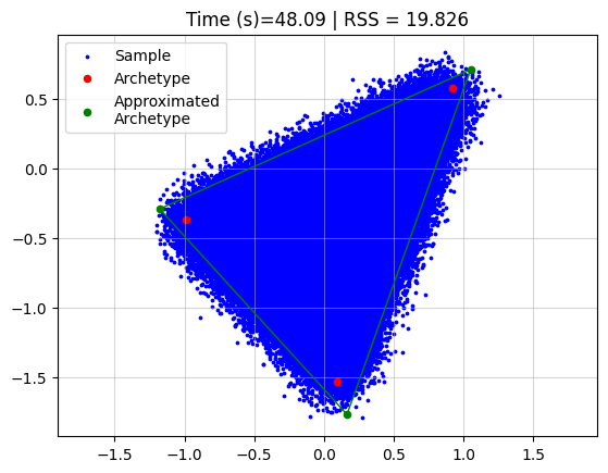
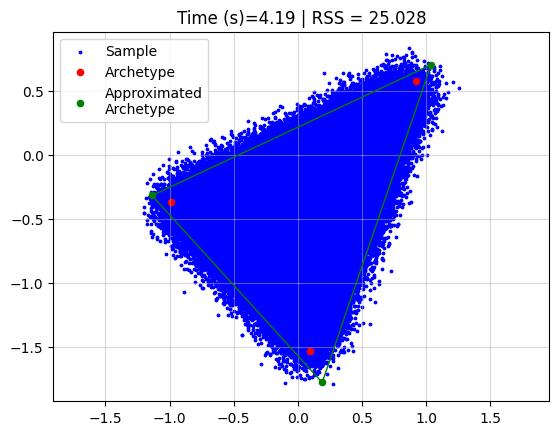
However, if we use coresets we can drastically reduce the time, without affecting the reconstruction a lot.

start = datetime.now()
AA_object = pt.AA(n_archetypes=3, coreset_algorithm="standard", coreset_fraction=0.05)
AA_object.fit(X)
Z_hat = AA_object.Z
end = datetime.now()
time = (end - start).total_seconds()

plt.grid(alpha=0.5)
plt.scatter(x=X[:, 0], y=X[:, 1], s=3, c="blue", label="Sample")
plt.scatter(x=Z[:, 0], y=Z[:, 1], s=20, c="red", label="Archetype")
plt.scatter(x=Z_hat[:, 0], y=Z_hat[:, 1], s=20, c="green", label="Approximated\nArchetype")
Z_loop = np.vstack([Z_hat, Z_hat[0]])
plt.plot(Z_loop[:, 0], Z_loop[:, 1], c="green", linestyle='-', linewidth=1)
plt.title(f"Time (s)={time:.2f} | RSS = {AA_object.RSS:.3f}")
plt.legend()
plt.axis("equal")
plt.show()