Quickstart

Packages

Note: To run the spatial analysis at the end of this tutorial you will need to install ParTIpy with the tutorial extras: pip install partipy[extra].

from pathlib import Path

import scanpy as sc
import pandas as pd
import plotnine as pn
import decoupler as dc
import numpy as np
from scipy.spatial.distance import cdist

import partipy as pt

Note: Importing partipy for the first time after installing might take some time (~30s) because numba needs to compile some code in the background. After that, it’ll be quick!

Data

First, we need to load and cache a single-cell dataset. In this example, we use mouse hepatocytes profiled by scRNA-seq from [BenMosheVM+22]. We downloaded the raw data from Zenodo and saved it to figshare for convenient access in this tutorial.

adata = sc.read("data/hepatocyte_processed.h5ad", backup_url="https://figshare.com/ndownloader/files/59459459")
adata

AnnData object with n_obs × n_vars = 1999 × 8354
    obs: 'cell_type', 'zone', 'run_id', 'time_point', 'UMAP_X', 'UMAP_Y'

Preprocessing

Before conducting archetypal analysis (AA) on single-cell RNA-seq data, it is beneficial to reduce the dimensionality of the data, as this helps remove noise and substantially increases the computational efficiency of AA. To achieve this, we first scale the counts across all cells to a common value using sc.pp.normalize_total, followed by logarithmic normalization with sc.pp.log1p.
By default, normalize_total scales each cell to the median total counts across all cells, which preserves the typical range of expression values prior to logarithmic transformation.

Next, we identify highly variable genes and apply principal component analysis (PCA) using only these genes.
All preprocessing steps are performed using functions from the scanpy package.

sc.pp.normalize_total(adata)
sc.pp.log1p(adata)
sc.pp.highly_variable_genes(adata)
sc.pp.pca(adata, mask_var="highly_variable")
adata.layers["z_scaled"]= sc.pp.scale(adata.X, max_value=10, copy=True)
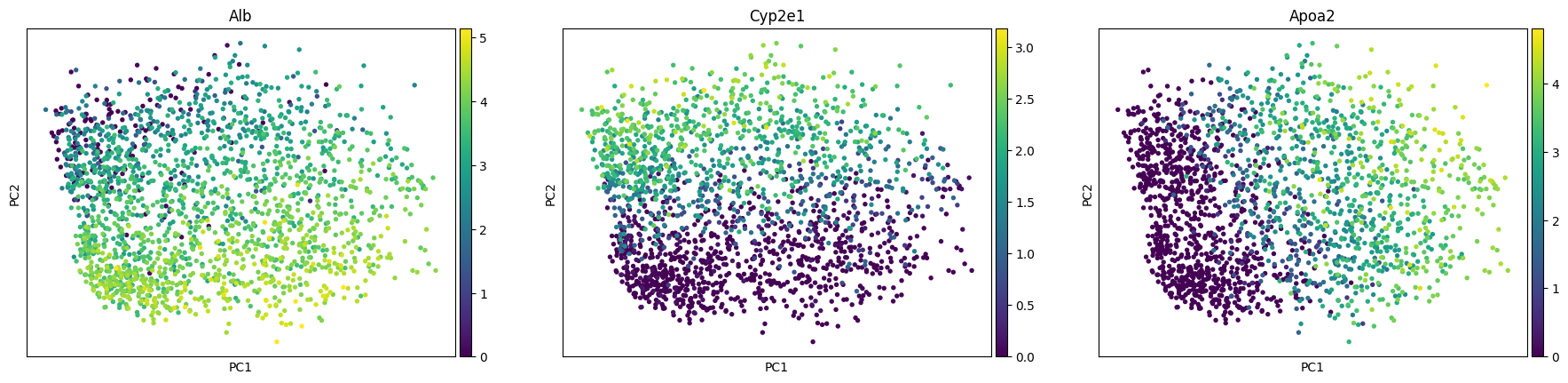
sc.pl.pca_scatter(adata, color=["Alb", "Cyp2e1", "Apoa2"])

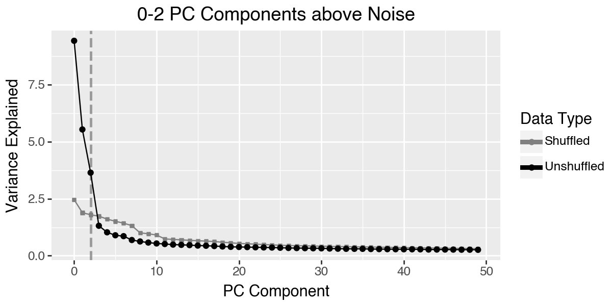
To determine the number of principal components to use for fitting the archetypes, we will examine the scree plot from the PCA. Additionally the plot shows the variance explained if we shuffle the data before computing the PCA. This plot indicates that we should only use the first three principal components.

pt.compute_shuffled_pca(adata, mask_var="highly_variable")
pt.plot_shuffled_pca(adata)

We store this setting in the adata.uns slot using the utility function set_obsm. Using n_dimensions=3 is equivalent to specifiy n_dimensions=[0, 1, 2]. If you do not want to use the first princial component, for example because it captures some technical effect, then you can simply specify n_dimensions=[1, 2].

pt.set_obsm(adata=adata, obsm_key="X_pca", n_dimensions=3)

Choosing the Number of Archetypes

Now, we are ready to perform archetypal analysis, but the key question remains: how many archetypes should be used?

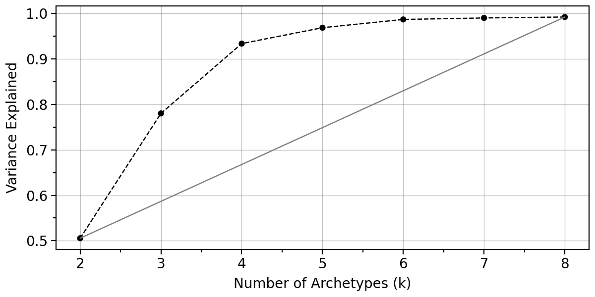
There is no definitive ground truth for this choice, but several heuristics can guide the decision. One approach is to evaluate how much variance is explained by different numbers of archetypes.

The function var_explained_aa() takes the reduced PCA data and computes the explained variance across a range of archetypes (from min_k to max_k). By default, this function utilizes all available CPU cores, as indicated by the n_jobs argument, which is set to -1.

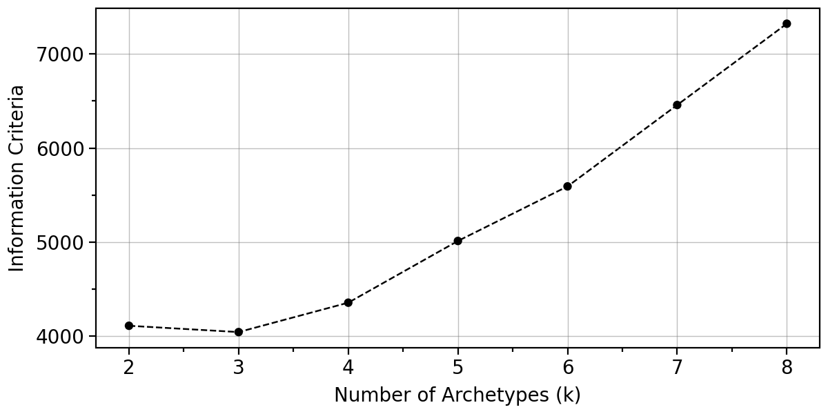
Additionally the function var_explained_aa() computes an information criteria which was suggested by Suleman, A., 2017. Validation of archetypal analysis, in: 2017 IEEE International Conference on Fuzzy Systems (FUZZ-IEEE) pp. 1–6. https://doi.org/10.1109/FUZZ-IEEE.2017.8015385

The results are stored in adata.uns["AA_metrics"] and can be effectively visualized using plot_var_explained_aa(). The plot suggests that a reasonable choice for the number of archetypes is 4 as the additional explained variance becomes negligible beyond this point.

adata

AnnData object with n_obs × n_vars = 1999 × 8354
    obs: 'cell_type', 'zone', 'run_id', 'time_point', 'UMAP_X', 'UMAP_Y'
    var: 'highly_variable', 'means', 'dispersions', 'dispersions_norm'
    uns: 'log1p', 'hvg', 'pca', 'AA_pca', 'AA_config'
    obsm: 'X_pca'
    varm: 'PCs'
    layers: 'z_scaled'

pt.compute_selection_metrics(adata=adata, n_archetypes_list=range(2, 9))
pt.plot_var_explained(adata)

pt.plot_IC(adata)

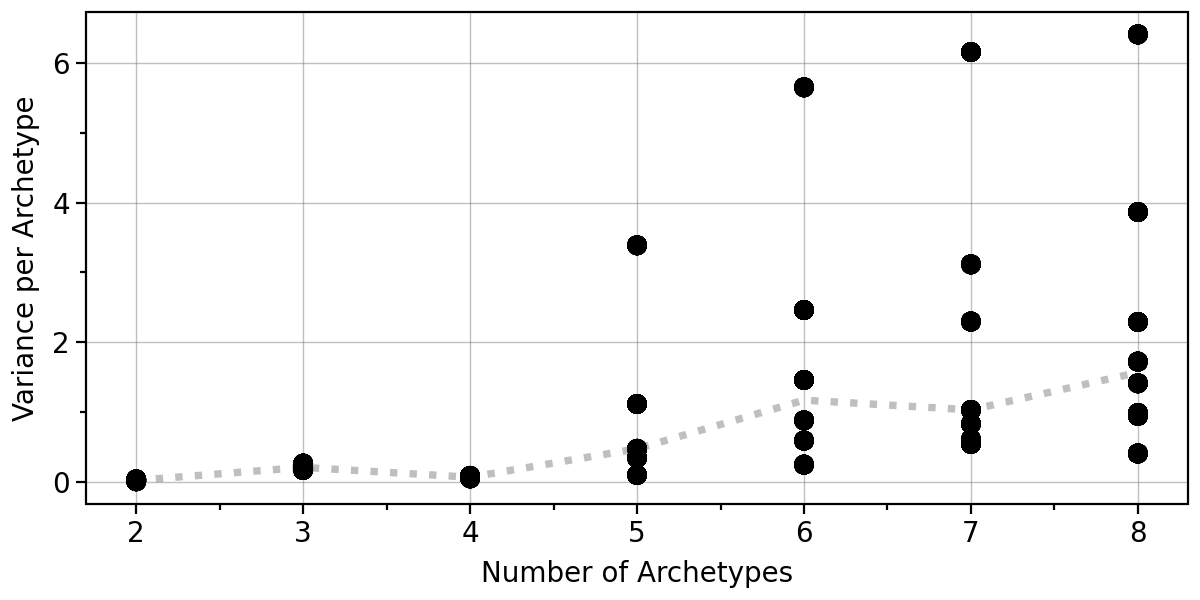
An important consideration is whether the positions of the archetypes remain stable for a given number of archetypes. To assess this, we apply bootstrapping and perform Archetypal Analysis (AA) on resampled datasets.

By default, this function utilizes all available CPU cores, as specified by the n_jobs argument, which is set to -1. The results are stored in adata.uns["AA_bootstrap"] and can be visualized using pt.plot_bootstrap_variance(adata).

As hinted to above, this result also suggest that 4 archetypes are highly stable.

pt.compute_bootstrap_variance(adata=adata, n_bootstrap=50, n_archetypes_list=range(2, 9))
pt.plot_bootstrap_variance(adata)

Archetypal Analysis

To compute the archetypes, we can simply use the compute_archetypes function. There are many optimization parameters which we describe in more detail in the vignette about Archetypal Analysis. We only briefly demonstrate how results from archetypal analysis can be incorporated when varying parameters, using the delta parameter as an example.

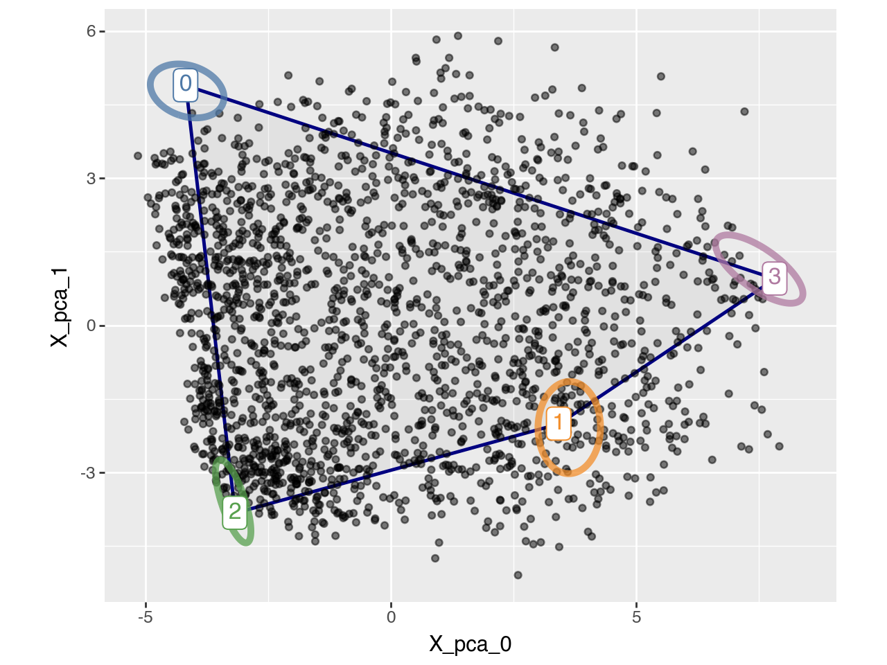
To get a feeling for the archetypes we might plot the polytope on first two dimensions. However, note that we actually fitted the polytope in a higher dimensional space.

#pt.compute_archetypes(adata, n_archetypes=4, archetypes_only=False)
pt.plot_archetypes_2D(adata=adata, show_contours=True, result_filters={"n_archetypes": 4, "delta": 0.0})

When only a few cells are sampled near the boundaries of the true phenotypic space, the convex hull of the observed data may underestimate the full range of variation. Such limited sampling can occur, for example, when the sample size is small or when the population is dominated by generalist cells rather than task-specialized ones. In these cases, relaxing the convexity constraint can help recover the true archetypes. This is achieved by introducing a relaxation parameter delta (see Equation 2 in the preprint), where larger delta values allow archetypes to lie farther from the data cloud (see Supplementary Figure S1 in the preprint). This approach has been used in [KSH+15] and subsequent works. The corresponding plot for delta=0.5 is shown below.

Whenever multiple archetypal analysis results are stored in adata.uns["AA_results"], the result_filters dictionary must be used to uniquely identify which result (e.g., combination of n_archetypes and delta) to visualize or analyze. This argument is consistently required in all subsequent functions.

#pt.compute_archetypes(adata, n_archetypes=4, delta=0.5, archetypes_only=False)
pt.compute_bootstrap_variance(adata=adata, n_bootstrap=50, n_archetypes_list=[4], delta=0.5)
pt.plot_archetypes_2D(adata=adata, show_contours=True, result_filters={"n_archetypes": 4, "delta": 0.5})

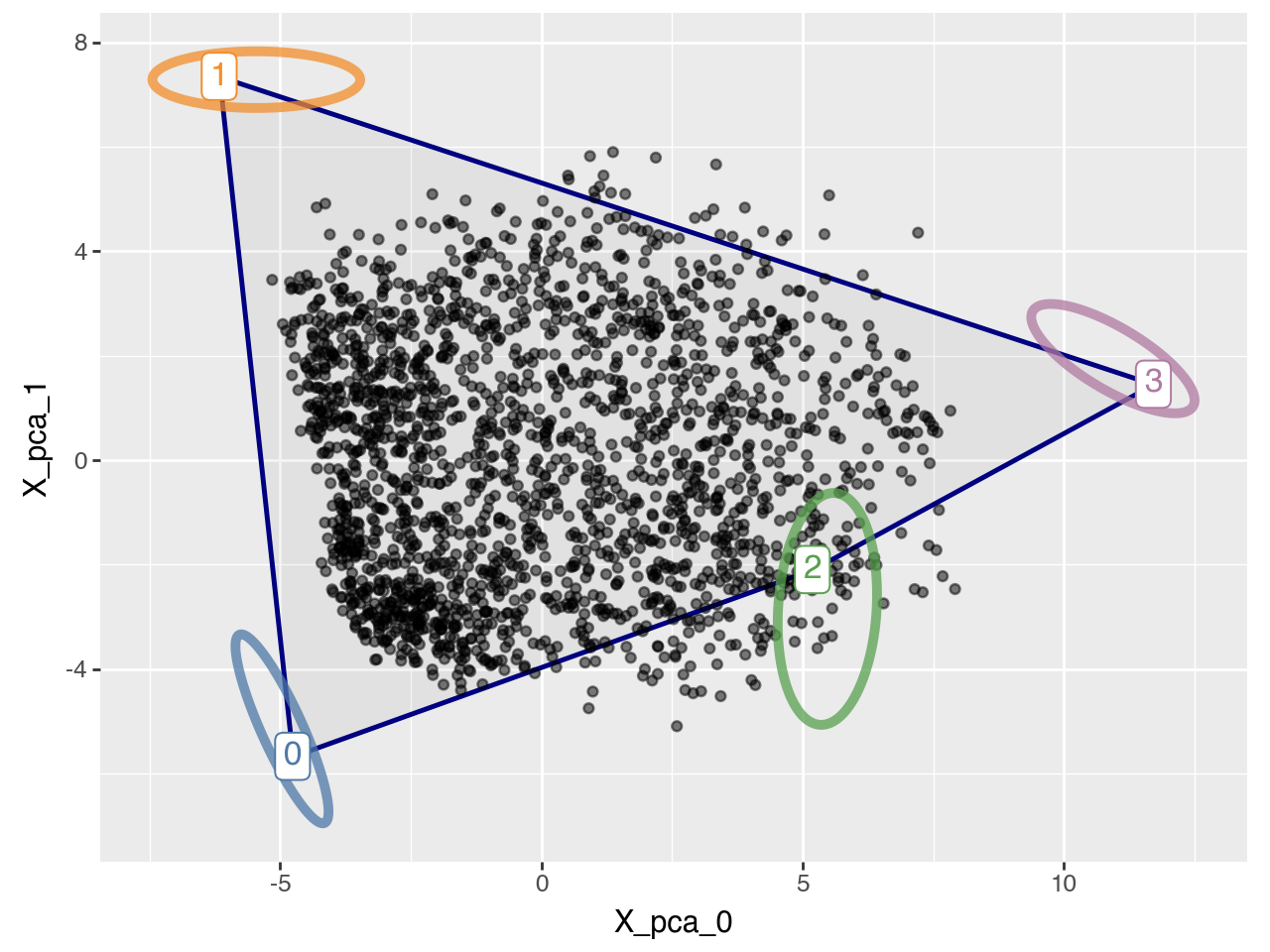
For simplicity in this quickstart example, we will continue using delta = 0.0.

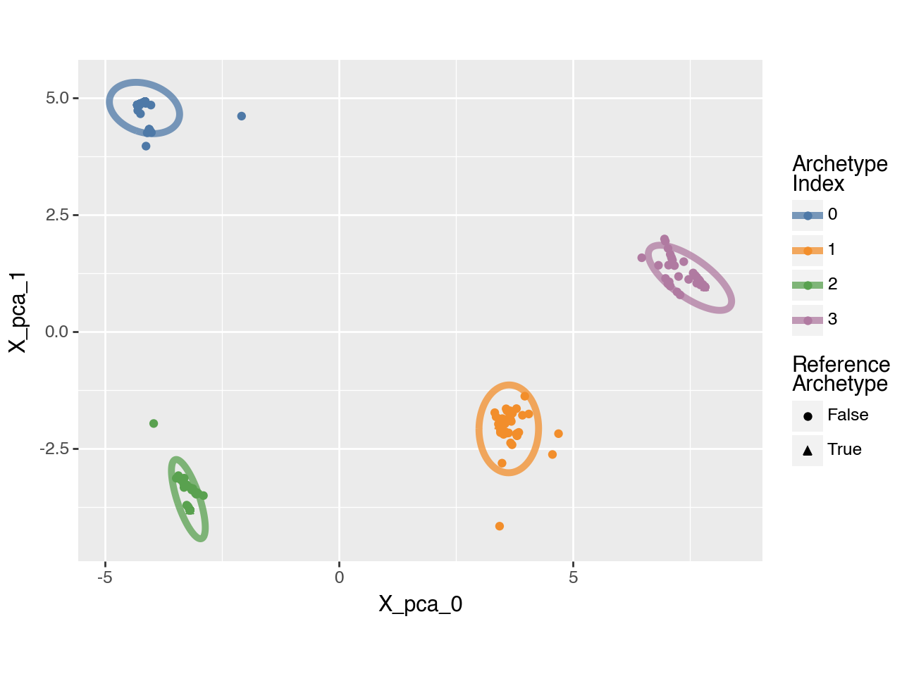
For a given \(k\) we can also visually asses the bootstrap stability using pt.plot_bootstrap_2D(adata) for the first two principal components and pt.plot_bootstrap_3D(adata) for the first three.

Since Plotly does not render properly when exporting Jupyter notebooks, we will use only the 2D scatter plot here.

#pt.plot_bootstrap_3D(adata, result_filters={"n_archetypes": 4})
pt.plot_bootstrap_2D(adata, result_filters={"n_archetypes": 4, "delta": 0.0})

We can assess statistical significance by permuting the principal component (PC) coordinates and evaluating whether the polytope fit is worse on the permuted data than on the original data. To quantify the goodness of fit, we can use the residual sum of squares (RSS), which yields a p-value of 0.0 in this case. Alternatively, we can use the ratio between the volume of the convex hull of the archetypes and that of the data, and assess whether this ratio is closer to 1 for the original data than for the permuted data. In this case, the resulting p-value is 0.13.

significance = pt.t_ratio_significance(adata, result_filters={"n_archetypes": 4, "delta": 0.0})
significance

{'t_ratio_p_value': np.float64(0.13), 'rss_p_value': np.float64(0.0)}

Below, we will focus on the archetype that is enriched in detoxification functions.

arch_idx = 0

Characterizing Archetypes

To better understand the archetypes, we aim to obtain the characteristic gene expression profile for each one.

We begin by computing the archetypal weights using the compute_archetype_weights() function, which assigns each cell a weight for each archetype based on its proximity to the archetype in the reduced space.

Next, we generate a the characteristic expression profile for each archetype using weighted averaging. This is achieved with the compute_archetype_expression() function, which aggregates expression data across cells according to their archetypal contributions.

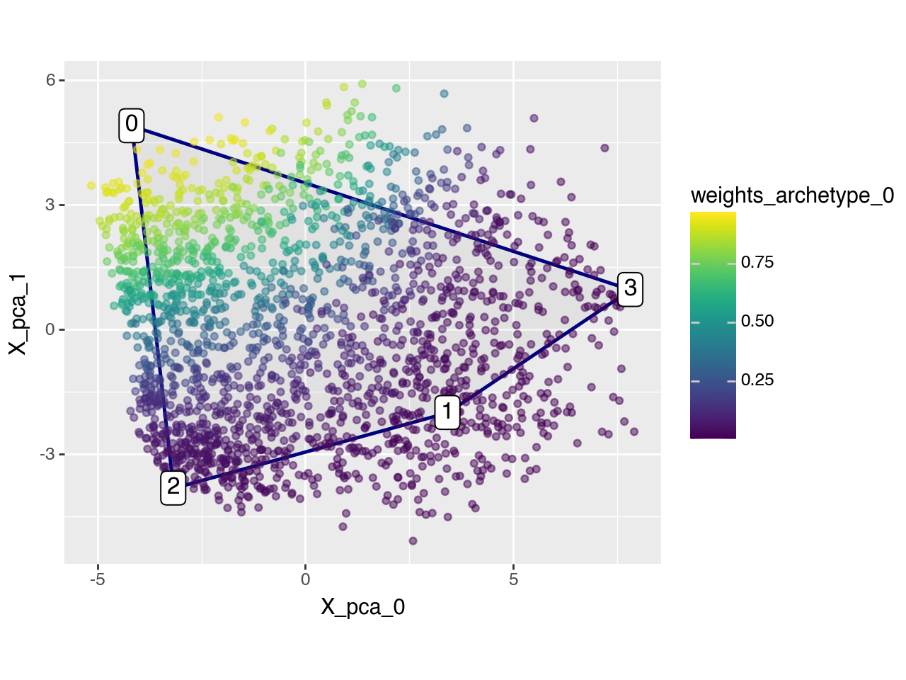
To better illustrate this, we visualize the weights for archetype 0 using the plot_2D_adata() function, highlighting the extent to which each cell is associated with it.

pt.compute_archetype_weights(adata=adata, mode="automatic", result_filters={"n_archetypes": 4, "delta": 0.0})
archetype_expression = pt.compute_archetype_expression(adata=adata, layer="z_scaled", result_filters={"n_archetypes": 4, "delta": 0.0})

adata.obs[f"weights_archetype_{arch_idx}"] = pt.get_aa_cell_weights(adata, n_archetypes=4, delta=0.0)[:, arch_idx]
pt.plot_archetypes_2D(adata=adata, color=f"weights_archetype_{arch_idx}", result_filters={"n_archetypes": 4, "delta": 0.0})

Applied length scale is 3.25.

Now we can use the characteristic gene expression profile to see which genes are relatively important for each archetype. As promised above, archetype 0 is characterized by high expression of Cytochrome P450 enzymes which are important for detoxification.

archetype_expression.T.sort_values(arch_idx, ascending=False).head(10)

	0	1	2	3
Cyp2e1	436.020325	-30.197796	-363.708191	-42.114399
Cyp2c29	365.530182	17.925915	-330.889679	-52.566467
Oat	361.276886	-51.621613	-238.374237	-71.281128
Rgn	349.183044	-93.312042	-211.860992	-44.009998
Cyp2c50	341.633850	-17.005131	-281.102234	-43.526714
Cyp3a11	328.088959	-27.827208	-207.940628	-92.320992
Acaa1b	309.286926	-30.886375	-238.255859	-40.144562
Csad	306.864197	-118.296616	-158.174042	-30.393387
Cyp1a2	303.983734	-37.028790	-232.198242	-34.756485
Cyp4a10	303.701508	-44.637718	-179.192703	-79.871132

We can also use the characteristic gene expression profiles of each archetype to perform enrichment analysis with decoupler. Here, we focus on Reactome pathways because we are interested in metabolic processes.

database = "reactome_pathways"
min_genes_per_pathway = 5
max_genes_per_pathway = 80

# dc.op.resource("SIGNOR", organism="mouse")
msigdb_raw = dc.op.resource("MSigDB")
msigdb = msigdb_raw[msigdb_raw["collection"]==database]
selection_vec = ~ np.array(["RESPONSE_TO" in s for s in msigdb["geneset"]]) & \
    ~ np.array(["GENE_EXPRESSION" in s for s in msigdb["geneset"]]) & \
    ~ np.array(["SARS_COV" in s for s in msigdb["geneset"]]) & \
    ~ np.array(["STIMULATED_TRANSCRIPTION" in s for s in msigdb["geneset"]])
msigdb = msigdb.loc[selection_vec, :].copy()
msigdb = msigdb[~msigdb.duplicated(["geneset", "genesymbol"])].copy()
genesets_within_min = (msigdb.value_counts("geneset") >= min_genes_per_pathway).reset_index().query("count")["geneset"].to_list()
genesets_within_max = (msigdb.value_counts("geneset") <= max_genes_per_pathway).reset_index().query("count")["geneset"].to_list()
genesets_to_keep = list(set(genesets_within_min) & set(genesets_within_max))
msigdb = msigdb.loc[msigdb["geneset"].isin(genesets_to_keep), :].copy() # removing small gene sets
msigdb = msigdb.rename(columns={"geneset": "source", "genesymbol": "target"}) # required since decoupler >= 2.0.0
msigdb_mouse = dc.op.translate(msigdb, target_organism="mouse", columns=["target"]) # requires decoupler >= 2.0.0
msigdb_mouse = msigdb_mouse.drop_duplicates()

acts_ulm_est, acts_ulm_est_p = dc.mt.ulm(data=archetype_expression,
                                         net=msigdb_mouse,
                                         verbose=False)

acts_ulm_est.iloc[:4, :4]

	REACTOME_2_LTR_CIRCLE_FORMATION	REACTOME_ABACAVIR_ADME	REACTOME_ABC_TRANSPORTERS_IN_LIPID_HOMEOSTASIS	REACTOME_ABERRANT_REGULATION_OF_MITOTIC_EXIT_IN_CANCER_DUE_TO_RB1_DEFECTS
0	0.250352	0.536366	-1.368654	-0.038143
1	0.790421	0.030882	2.696743	0.205283
2	-0.654845	0.238214	-1.966948	-0.129916
3	-0.332060	-0.987200	1.611838	-0.018259

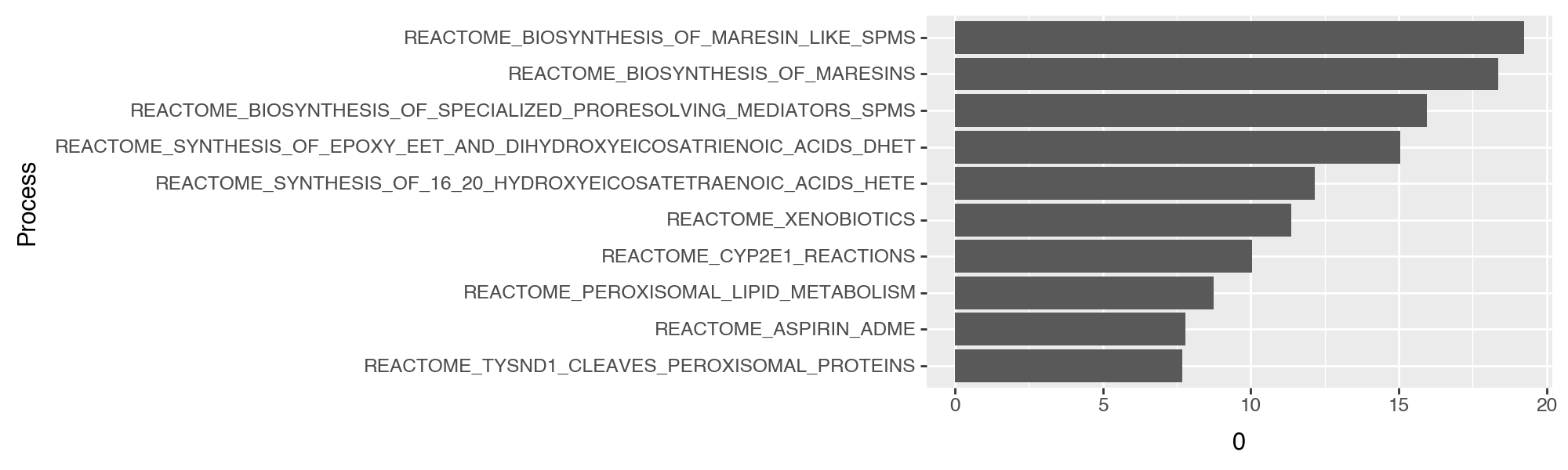
We can then extract the top \(x\) (here \(x=10\)) processes per archetype using extract_enriched_processes(). Focusing on Archetype 0 this revals Reactome pathways related to xenobiotics (including pathways related to oxidiaton and functionalization).

top_processes = pt.extract_enriched_processes(est=acts_ulm_est, 
                                              pval=acts_ulm_est_p, 
                                              order="desc", 
                                              n=10,
                                              p_threshold=0.05)
top_processes[0]

	Process	0	1	2	3	specificity
0	REACTOME_BIOSYNTHESIS_OF_MARESIN_LIKE_SPMS	19.231574	-0.073914	-17.587078	-3.201036	19.305488
1	REACTOME_BIOSYNTHESIS_OF_MARESINS	18.358449	-0.277203	-16.459156	-3.236373	18.635652
2	REACTOME_BIOSYNTHESIS_OF_SPECIALIZED_PRORESOLV...	15.946956	-0.924025	-13.981917	-2.451122	16.870981
3	REACTOME_SYNTHESIS_OF_EPOXY_EET_AND_DIHYDROXYE...	15.050412	-0.072619	-13.457143	-2.901618	15.123031
4	REACTOME_SYNTHESIS_OF_16_20_HYDROXYEICOSATETRA...	12.154629	0.060632	-10.380653	-3.082589	12.093997
5	REACTOME_XENOBIOTICS	11.373397	2.173401	-11.793349	-2.579222	9.199995
6	REACTOME_CYP2E1_REACTIONS	10.048127	2.525538	-10.734145	-2.557661	7.522589
7	REACTOME_PEROXISOMAL_LIPID_METABOLISM	8.744137	-2.767584	-5.231966	-1.933989	10.678127
8	REACTOME_ASPIRIN_ADME	7.787722	1.642602	-7.991403	-1.944230	6.145119
9	REACTOME_TYSND1_CLEAVES_PEROXISOMAL_PROTEINS	7.687111	-1.734316	-5.439395	-1.463540	9.150651

top_processes[arch_idx]["Process"] = pd.Categorical(
    top_processes[arch_idx]["Process"],
    categories=top_processes[arch_idx].sort_values(f"{arch_idx}", ascending=True)["Process"].to_list()
)

(pn.ggplot(top_processes[arch_idx])
 + pn.geom_col(pn.aes(x="Process", y=f"{arch_idx}"))
 + pn.coord_flip()
 + pn.theme(figure_size=(10, 3)))

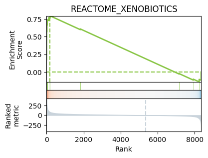
Then, we can decoupler’s leading edge function to check for example which genes have a high weight for our archetype of interest, and are in the gene set for “REACTOME_XENOBIOTICS”.

df = archetype_expression.T.copy()
df.columns = df.columns.astype(str)
_, le = dc.pl.leading_edge(
    df = df,
    net = msigdb_mouse,
    stat = str(arch_idx),
    name = "REACTOME_XENOBIOTICS"
)
print(le)

['Cyp2e1' 'Cyp2c29' 'Cyp2c50' 'Cyp1a2' 'Cyp2c37' 'Cyp2a5' 'Cyp2c38' 'Ahr']

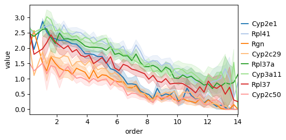
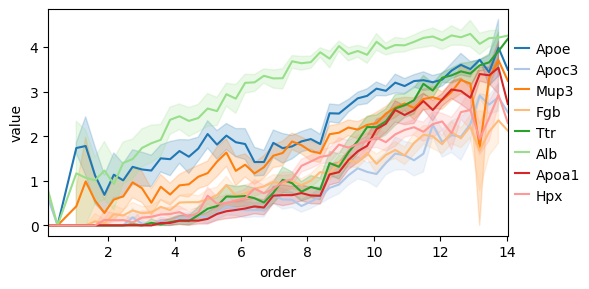
Another interesting thing we can do is to consider how gene expressions changes as a function of the distance to some archetype. To this end we can use the decoupler functions dc.tl.rankby_order, dc.pp.bin_order, and dc.pl.order.

Z = pt.get_aa_result(adata, n_archetypes=4, delta=0)["Z"]
distances = cdist(
    adata.obsm[adata.uns["AA_config"]["obsm_key"]][:, adata.uns["AA_config"]["n_dimensions"]],
    Z
)
for idx in range(Z.shape[1]):
    adata.obs[f"dist_to_arch_{idx}"] = distances[:, idx]

genes_ordered = dc.tl.rankby_order(
    adata=adata,
    order=f"dist_to_arch_{arch_idx}",
    stat="spearmanr",
)
top_genes = genes_ordered.sort_values("stat").head(8)["name"].to_list()
bottom_genes = genes_ordered.sort_values("stat").tail(8)["name"].to_list()

top_genes_ordered = dc.pp.bin_order(
    adata=adata,
    order=f"dist_to_arch_{arch_idx}",
    names=top_genes,
     nbins=50,
)

bottom_genes_ordered = dc.pp.bin_order(
    adata=adata,
    order=f"dist_to_arch_{arch_idx}",
    names=bottom_genes,
     nbins=50,
)

dc.pl.order(
    df=top_genes_ordered,
    mode="line",
    figsize=(6, 3),
)

dc.pl.order(
    df=bottom_genes_ordered,
    mode="line",
    figsize=(6, 3),
)

Alternatively, we can use the quantile-based, distance-ranking gene-enrichment algorithm used in previous ParTI work [AKKT+19, HSH+15, KSH+15] (see Supplementary Methods Section 4.4), which tests for genes whose expression is highest in the quantile bin closest to an archetype relative to a background (by default all remaining cells, with optional alternative contrasts such as closest versus furthest bins). This algorithm is implemented in pt.compute_quantile_based_gene_enrichment.

However note that this approach requires per-gene and per-archetype hypothesis testing across large numbers of cells and therefore scales less well than kernel-aggregated profiling.

gene_enrichment = pt.compute_quantile_based_gene_enrichment(adata, result_filters={"n_archetypes": 4, "delta": 0.0})
gene_enrichment.query("enriched").query(f"arch_idx=={arch_idx}").sort_values("pval_adj").head(6)

	arch_idx	gene	stat	pval	mean_diff	median_diff	mean_bin0	mean_rest	median_bin0	median_rest	max_in_bin0	pos_effect	pval_adj	signif	enriched
3779	0	Oat	306028.5	7.122084e-85	0.998351	1.177536	1.253019	0.254668	1.177536	0.000000	True	True	5.949789e-81	True	True
3801	0	Cyp2e1	315818.0	3.467040e-73	1.352518	2.014842	2.181629	0.829111	2.221061	0.206219	True	True	9.654550e-70	True	True
8235	0	Cyp2c50	289663.0	1.178018e-48	0.678192	0.807465	1.207931	0.529739	1.236465	0.429001	True	True	1.968233e-45	True	True
4263	0	Rpl41	293127.0	1.654406e-48	0.871232	0.713324	2.552605	1.681374	2.618408	1.905084	True	True	2.303484e-45	True	True
8227	0	Cyp2c29	290362.5	2.534837e-48	0.896444	1.324256	1.629166	0.732722	1.712150	0.387894	True	True	3.025147e-45	True	True
2009	0	Cyp4a10	272953.0	4.374906e-48	0.541017	0.781933	0.764036	0.223019	0.781933	0.000000	True	True	4.568496e-45	True	True

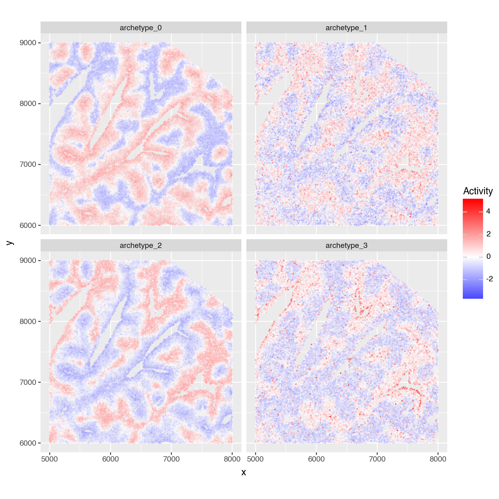
Spatial Enrichment

As in [AKKT+19], we want to quantify where the archetypes locate in the tissue.

To that end we download a single-cell spatial data set from the liver from https://info.vizgen.com/mouse-liver-data (Vizgen MERFISH Mouse Liver Map January 2022). In particular we only need to download from Liver1Slice1 the files "cell_by_gene.csv", "cell_metadata.csv" and place those in the folder Liver1Slice1 in data.

Then, to quantify to which archetype any given cell is close to, we compute the enrichment of the archetype gene expression signatures in each cells’ gene expression profile.

import sys
!{sys.executable} -m pip install --quiet squidpy

# only run if the data has actually been downloaded
if (Path(".") / "data" / "Liver1Slice1" / "Liver1Slice1_cell_by_gene.csv").exists() and (Path(".") / "data" / "Liver1Slice1" / "Liver1Slice1_cell_metadata.csv").exists():
    import squidpy as sq
    vizgen_adata = sq.read.vizgen(
        "./data/Liver1Slice1",
        counts_file="Liver1Slice1_cell_by_gene.csv",
        meta_file="Liver1Slice1_cell_metadata.csv",
    )
    vizgen_adata = vizgen_adata[:, vizgen_adata.var.index.isin(archetype_expression.columns.to_list())].copy()
    vizgen_adata = vizgen_adata[vizgen_adata.X.sum(axis=1).A1 > 200, :].copy()
    sc.pp.normalize_total(vizgen_adata)
    sc.pp.log1p(vizgen_adata)

    # create weights based on archetype expression profile
    archetype_expression_weights = (archetype_expression[vizgen_adata.var.index].copy()
                                    .reset_index(names="archetype")
                                    .melt(id_vars="archetype", value_name="weight", var_name="gene")
                                    )
    archetype_expression_weights = archetype_expression_weights.rename(columns={"archetype": "source", "gene": "target"})

    # compute the enrichment of the archetype gex profiles in the gex profiles of each cell
    dc.mt.ulm(data=vizgen_adata, net=archetype_expression_weights, verbose=False)

    # plotting one part
    plotting_df = vizgen_adata.obsm["score_ulm"].copy()
    plotting_df.columns = ["archetype_" + idx for idx in plotting_df.columns]
    plotting_df = plotting_df - plotting_df.mean()
    plotting_df = plotting_df / plotting_df.std()
    plotting_df["x"] = vizgen_adata.obsm["spatial"][:, 0]
    plotting_df["y"] = vizgen_adata.obsm["spatial"][:, 1]

    width = 3_000
    x_low = 5_000
    y_low = 6_000
    x_high = x_low + width
    y_high = y_low + width
    plotting_df = plotting_df.loc[(plotting_df["x"] > x_low) & (plotting_df["x"] < x_high) & (plotting_df["y"] > y_low) & (plotting_df["y"] < y_high)]

    plotting_df = plotting_df.melt(id_vars=["x", "y"], value_name="score", var_name="archetype")
    p = (pn.ggplot(plotting_df) 
        + pn.geom_point(pn.aes(x="x", y="y", color="score"), size=0.1, alpha=0.5) 
        + pn.scale_color_gradient2(low="blue", mid="white", high="red", midpoint=0)
        + pn.facet_wrap(facets="archetype", nrow=2, ncol=2)
        + pn.coord_equal() 
        + pn.theme(figure_size=(8, 8)) 
        + pn.labs(x="x", y="y", color="Activity")
        )
    p.show()

Saving and Loading Results

See more details in the Accessing And Saving Cached Results vignette vignette. In brief: ParTIpy caches AA outputs with immutable ArchetypeConfig keys (a frozen Pydantic model), those objects keep the cache hashable inside adata.uns. HDF5 only accepts string keys, so pt.write_h5ad turns each config into a JSON string before writing, and pt.read_h5ad restores the original ArchetypeConfig objects so cached metrics still work after reloading.

pt.write_h5ad(adata, "adata.h5ad")
adata = pt.read_h5ad("adata.h5ad")
adata

AnnData object with n_obs × n_vars = 1999 × 8354
    obs: 'cell_type', 'zone', 'run_id', 'time_point', 'UMAP_X', 'UMAP_Y', 'weights_archetype_0', 'dist_to_arch_0', 'dist_to_arch_1', 'dist_to_arch_2'
    var: 'highly_variable', 'means', 'dispersions', 'dispersions_norm'
    uns: 'AA_bootstrap', 'AA_cell_weights', 'AA_config', 'AA_pca', 'AA_results', 'AA_selection_metrics', 'AA_t_ratio', 'hvg', 'log1p', 'pca'
    obsm: 'X_pca'
    varm: 'PCs'
    layers: 'z_scaled'

Session Info

import session_info2
print(session_info2.session_info(dependencies=True))

pandas	2.2.3
scanpy	1.11.2
plotnine	0.14.5
decoupler	2.0.6
numpy	2.2.6
scipy	1.15.2
partipy	0.0.5 (0.0.1)
anndata	0.11.4
squidpy	1.6.5
----	----
networkx	3.5
jupyter_client	8.6.3
dcor	0.6
wrapt	1.17.2
matplotlib	3.10.3
requests	2.32.3
zipp	3.22.0
asttokens	3.0.0
igraph	0.11.8
asciitree	0.3.3
texttable	1.7.0
ipywidgets	8.1.7
typing_extensions	4.15.0
pydantic_core	2.41.1
statsmodels	0.14.4
session-info2	0.1.2
pyzmq	26.4.0
threadpoolctl	3.6.0
multipledispatch	1.0.0 (0.6.0)
idna	3.10
multiscale_spatial_image	2.0.2
pyproj	3.7.1
h5py	3.13.0
shapely	2.1.1
traitlets	5.14.3
tqdm	4.67.1
pillow	11.2.1
packaging	25.0
adjustText	1.3.0
legendkit	0.3.5
six	1.17.0
charset-normalizer	3.4.2
decorator	5.2.1
debugpy	1.8.14
xarray-schema	0.0.3
zstandard	0.25.0
ipython	9.2.0
wcwidth	0.2.13
spatialdata	0.4.0
numba	0.61.2
typing-inspection	0.4.2
pexpect	4.9.0
xgboost	3.0.2
dask	2024.11.2
imageio	2.37.0
dask-image	2024.5.3
pyct	0.5.0
jedi	0.19.2
docrep	0.3.2
attrs	25.3.0
pytz	2025.2
annotated-types	0.7.0
comm	0.2.2
certifi	2025.4.26 (2025.04.26)
ptyprocess	0.7.0
matplotlib-scalebar	0.9.0
geopandas	1.0.1
llvmlite	0.44.0
platformdirs	4.3.8
python-dateutil	2.9.0.post0
marsilea	0.5.3
cycler	0.12.1
pure_eval	0.2.3
cloudpickle	3.1.1
natsort	8.4.0
legacy-api-wrap	1.4.1
appnope	0.1.4
patsy	1.0.1
pydantic	2.12.0
executing	2.2.0
crc32c	2.7.1
jaraco.context	6.0.1
plotly	6.1.2
mizani	0.13.5
spatial_image	1.2.1
xarray-spatial	0.4.0
param	2.2.0
validators	0.35.0
jaraco.classes	3.4.0
Pygments	2.19.1
jaraco.text	3.12.1
seaborn	0.13.2
rich	14.0.0
scikit-image	0.25.2
PyYAML	6.0.2
coverage	7.10.7
xarray	2024.11.0
more-itertools	10.7.0
importlib_metadata	8.7.0
pyparsing	3.2.3
Deprecated	1.2.18
numcodecs	0.15.1
jaraco.functools	4.3.0
joblib	1.5.1
ome-zarr	0.11.1
matplotlib-inline	0.1.7
tifffile	2025.5.26
jupyter_core	5.8.1
scikit-learn	1.6.1
tornado	6.5.1
urllib3	2.4.0
parso	0.8.4
xarray-dataclasses	1.9.1
pyarrow	20.0.0
zarr	2.18.7
jaraco.collections	5.1.0
stack-data	0.6.3
narwhals	1.41.0
fsspec	2025.5.1
colorama	0.4.6
lazy_loader	0.4
datashader	0.18.1
setuptools	80.8.0
kiwisolver	1.4.8
toolz	1.0.0
prompt_toolkit	3.0.51
ipykernel	6.29.5
psutil	7.0.0
----	----
Python	3.11.0 | packaged by conda-forge | (main, Jan 14 2023, 12:26:40) [Clang 14.0.6 ]
OS	macOS-15.7.1-arm64-arm-64bit
Updated	2026-01-31 15:52