Archetypal Analysis

Introduction

In this vignette, we present

1. a brief overview of the theory behind archetypal analysis

2. a description of the optimization procedure used in our implementation

3. a guide to using the AA class and its AA.fit() method

First, we will import some package that we need throughout this vignette.

from datetime import datetime
import partipy as pt
import numpy as np
import matplotlib.pyplot as plt

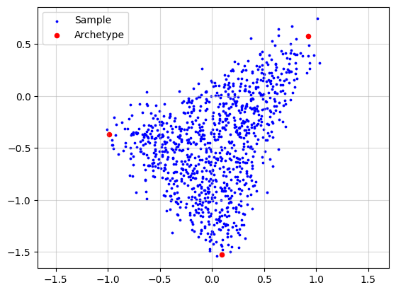
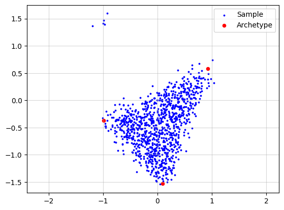
Now, we simulate a dataset to provide an intuitive explanation of archetypal analysis. To make the simulation more realistic, we add noise to each data point by sampling a noise vector from an isotropic Gaussian distribution.

X, A, Z = pt.simulate_archetypes(n_samples=1_000, n_archetypes=3, n_dimensions=2, 
                                 noise_std=0.10, seed=123)
print(f"{X.shape}")
print(f"{A.shape}")
print(f"{Z.shape}")

(1000, 2)
(1000, 3)
(3, 2)

plt.grid(alpha=0.5)
plt.scatter(x=X[:, 0], y=X[:, 1], s=3, c="blue", label="Sample")
plt.scatter(x=Z[:, 0], y=Z[:, 1], s=20, c="red", label="Archetype")
plt.legend()
plt.axis("equal")
plt.show()

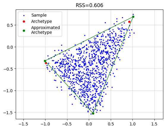
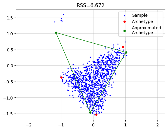
Standard Archetypal Analysis

To recover the archetypes we simply need to call

AA_object = pt.AA(n_archetypes=3)
AA_object.fit(X)
Z_hat = AA_object.Z

plt.grid(alpha=0.5)
plt.scatter(x=X[:, 0], y=X[:, 1], s=3, c="blue", label="Sample")
plt.scatter(x=Z[:, 0], y=Z[:, 1], s=20, c="red", label="Archetype")
plt.scatter(x=Z_hat[:, 0], y=Z_hat[:, 1], s=20, c="green", label="Approximated\nArchetype")
Z_loop = np.vstack([Z_hat, Z_hat[0]])
plt.plot(Z_loop[:, 0], Z_loop[:, 1], c="green", linestyle='-', linewidth=1)
plt.title(f"RSS={AA_object.RSS:.3f}")
plt.legend()
plt.axis("equal")
plt.show()

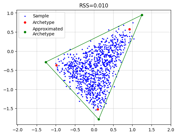
Relaxation of Convex Constraint on Archetypes

AA_object = pt.AA(n_archetypes=3, delta=0.25)
AA_object.fit(X)
Z_hat = AA_object.Z

plt.grid(alpha=0.5)
plt.scatter(x=X[:, 0], y=X[:, 1], s=3, c="blue", label="Sample")
plt.scatter(x=Z[:, 0], y=Z[:, 1], s=20, c="red", label="Archetype")
plt.scatter(x=Z_hat[:, 0], y=Z_hat[:, 1], s=20, c="green", label="Approximated\nArchetype")
Z_loop = np.vstack([Z_hat, Z_hat[0]])
plt.plot(Z_loop[:, 0], Z_loop[:, 1], c="green", linestyle='-', linewidth=1)
plt.title(f"RSS={AA_object.RSS:.3f}")
plt.legend()
plt.axis("equal")
plt.show()

Robust Archetypal Analysis

To demonstrate robust archetypal anaysis we will add some outliers here.

n_outliers = 5
outlier_mean = np.array([-1.0, 1.5])
X_wo = np.zeros((X.shape[0]+n_outliers, X.shape[1]))
X_wo[:X.shape[0], :] = X.copy()
rng = np.random.default_rng(seed=42)
X_wo[X.shape[0]:, :] = rng.normal(loc=outlier_mean, scale=(0.1, 0.1), size=(n_outliers, 2))

print(f"{X_wo.shape}")
print(f"{A.shape}")
print(f"{Z.shape}")

(1005, 2)
(1000, 3)
(3, 2)

plt.grid(alpha=0.5)
plt.scatter(x=X_wo[:, 0], y=X_wo[:, 1], s=3, c="blue", label="Sample")
plt.scatter(x=Z[:, 0], y=Z[:, 1], s=20, c="red", label="Archetype")
plt.legend()
plt.axis("equal")
plt.show()

Now if we just run the standard algorithm we obtain.

AA_object = pt.AA(n_archetypes=3)
AA_object.fit(X_wo)
Z_hat = AA_object.Z

plt.grid(alpha=0.5)
plt.scatter(x=X_wo[:, 0], y=X_wo[:, 1], s=3, c="blue", label="Sample")
plt.scatter(x=Z[:, 0], y=Z[:, 1], s=20, c="red", label="Archetype")
plt.scatter(x=Z_hat[:, 0], y=Z_hat[:, 1], s=20, c="green", label="Approximated\nArchetype")
Z_loop = np.vstack([Z_hat, Z_hat[0]])
plt.plot(Z_loop[:, 0], Z_loop[:, 1], c="green", linestyle='-', linewidth=1)
plt.title(f"RSS={AA_object.RSS:.3f}")
plt.legend()
plt.axis("equal")
plt.show()

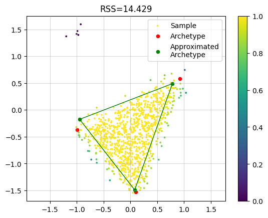
However, if we use the robust implementation we get a much better result. In the plot we colored each sample by the final weight. We see that the outlier samples have zero weight.

AA_object = pt.AA(n_archetypes=3, weight="bisquare", early_stopping=False)
AA_object.fit(X_wo)
Z_hat = AA_object.Z

plt.grid(alpha=0.5)
plt.scatter(x=X_wo[:, 0], y=X_wo[:, 1], s=3, c=AA_object.W, label="Sample")
plt.scatter(x=Z[:, 0], y=Z[:, 1], s=20, c="red", label="Archetype")
plt.scatter(x=Z_hat[:, 0], y=Z_hat[:, 1], s=20, c="green", label="Approximated\nArchetype")
Z_loop = np.vstack([Z_hat, Z_hat[0]])
plt.plot(Z_loop[:, 0], Z_loop[:, 1], c="green", linestyle='-', linewidth=1)
plt.title(f"RSS={AA_object.RSS:.3f}")
plt.legend()
plt.colorbar()
plt.axis("equal")
plt.show()

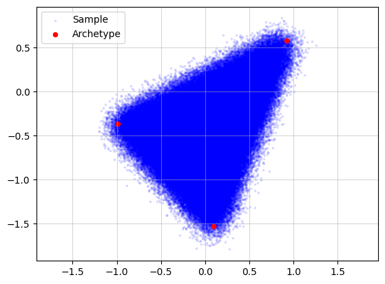
Coresets

Let’s use the same archetypes but generate much more samples.

X, A, Z = pt.simulate_archetypes(n_samples=200_000, n_archetypes=3, n_dimensions=2, 
                                 noise_std=0.10, seed=123)
print(f"{X.shape}")
print(f"{A.shape}")
print(f"{Z.shape}")

(200000, 2)
(200000, 3)
(3, 2)

plt.grid(alpha=0.5)
plt.scatter(x=X[:, 0], y=X[:, 1], s=3, c="blue", label="Sample", alpha=0.1)
plt.scatter(x=Z[:, 0], y=Z[:, 1], s=20, c="red", label="Archetype")
plt.legend()
plt.axis("equal")
plt.show()

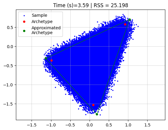
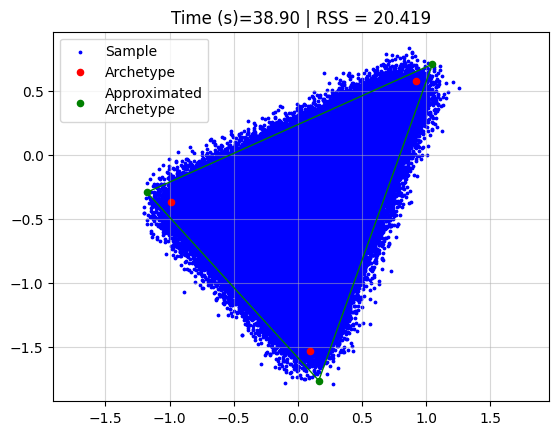
Running archetypal analysis now takes quite some time

start = datetime.now()
AA_object = pt.AA(n_archetypes=3)
AA_object.fit(X)
Z_hat = AA_object.Z
end = datetime.now()
time = (end - start).total_seconds()

plt.grid(alpha=0.5)
plt.scatter(x=X[:, 0], y=X[:, 1], s=3, c="blue", label="Sample")
plt.scatter(x=Z[:, 0], y=Z[:, 1], s=20, c="red", label="Archetype")
plt.scatter(x=Z_hat[:, 0], y=Z_hat[:, 1], s=20, c="green", label="Approximated\nArchetype")
Z_loop = np.vstack([Z_hat, Z_hat[0]])
plt.plot(Z_loop[:, 0], Z_loop[:, 1], c="green", linestyle='-', linewidth=1)
plt.title(f"Time (s)={time:.2f} | RSS = {AA_object.RSS:.3f}")
plt.legend()
plt.axis("equal")
plt.show()

However, if we use coresets we can drastically reduce the time, without affecting the performance a lot.

start = datetime.now()
AA_object = pt.AA(n_archetypes=3, coreset_algorithm="standard", coreset_fraction=0.05)
AA_object.fit(X)
Z_hat = AA_object.Z
end = datetime.now()
time = (end - start).total_seconds()

plt.grid(alpha=0.5)
plt.scatter(x=X[:, 0], y=X[:, 1], s=3, c="blue", label="Sample")
plt.scatter(x=Z[:, 0], y=Z[:, 1], s=20, c="red", label="Archetype")
plt.scatter(x=Z_hat[:, 0], y=Z_hat[:, 1], s=20, c="green", label="Approximated\nArchetype")
Z_loop = np.vstack([Z_hat, Z_hat[0]])
plt.plot(Z_loop[:, 0], Z_loop[:, 1], c="green", linestyle='-', linewidth=1)
plt.title(f"Time (s)={time:.2f} | RSS = {AA_object.RSS:.3f}")
plt.legend()
plt.axis("equal")
plt.show()